TL;DR Gradient descent updates weights, but the weight Gram matrix \(W^\top W\) records how the features would like to move.
Following that motion shows deep networks straightening their data toward the target, one layer at a time.
What if we moved the features instead?
Training changes weights. Now imagine a side experiment. Take an input \(x\), and at every training step
nudge a copy of it along the loss gradient, in the direction the loss would like the input to move:
We call \(\tilde x_t\) the virtual update. It never feeds back into training.
It is just a record of where gradient descent is pushing the features.
Below, a small MLP learns to predict each point's position along a Swiss roll (shown as color).
Press play and watch the record.
epoch 0
0.00Target Linearity of \(\tilde X_t\) (R² of linear regression \(\tilde X_t \to y\))
Training loss
The virtual update linearizes the data. Gray: original inputs \(X\). Color: virtually updated inputs \(\tilde X_t\).
On the Swiss roll, the spiral unrolls into a curve ordered by the target, and a plain linear regression from \(\tilde X_t\) to \(y\) goes from R² ≈ 0.07 to ≈ 1.00 over 100 epochs.
On two circles, the inner class is pulled out of the ring and the two classes end up on opposite sides (R² ≈ 0 → 0.95).
Swiss roll: full-batch GD with learning rate 0.2 and display step size \(\gamma = 700\) (setup as in Appendix B.1, trained longer and with a larger learning rate). Coordinates are min-max rescaled each frame for display; the dynamics are not.
The animation raises two questions, and the rest of this page answers them in order.
First, gradient descent only touches weights, so does it really carry this feature-space motion?
Second, where does the motion lead?
Pillar A · A feature-centric view
One line of chain rule connects weights to features
Most theories of training dynamics are weight-centric: they ask how far the weights move, as in NTK or mean-field analyses.
We ask instead how the features move. The bridge between the two views takes one line.
For any layer \(z = Wh\) and any scalar function \(f(z)\), the chain rule gives two gradients:
Feature gradient
\[ \nabla_{h} f = W^\top \nabla_{z} f \]
&
Weight gradient
\[ \nabla_{W} f = \nabla_{z} f\; h^\top \]
↓
The Feature Learning Equation
\[ \underbrace{\htmlClass{fx}{\nabla_{h} f \cdot h^\top}}_{\text{how features want to move}} \;=\; \underbrace{\htmlClass{wx}{W^\top \nabla_{W} f}}_{\text{how weights actually move}} \]
An exact identity, with no approximation. The two sides meet through \(W^\top\).
The Gram matrix is where feature gradients get written
Apply one gradient-descent step to \(W\), and look at the Gram matrix \(W^\top W\) rather than at \(W\) itself.
The Feature Learning Equation shows up inside the expansion:
The right-hand side contains no weight gradients, only feature gradients.
It is also exactly how the covariance \(hh^\top\) changes when \(h\) takes one virtual step \(h \to h - \gamma \nabla_h L\).
Theorem 1
The weight Gram matrix learns the Virtual Covariance.
Every gradient step shifts \(W^\top W\) by the same amount that the covariance of the virtually updated features shifts.
Gradient descent never moves features directly, yet the Gram matrix carries a record of where they were being pushed.
Show the math
With \(W^+ = W - \gamma\nabla_W L\) and virtual update \(h^+ = h - \gamma \nabla_h L\),
\[ (W^+)^\top W^+ - W^\top W \;=\; h^+ (h^+)^\top - h h^\top + O(\gamma^2). \]
Over a mini-batch, the per-sample shifts add up. Over \(\tau\) steps this gives
\(W_t^\top W_t - W_{t-\tau}^\top W_{t-\tau} \approx \tilde h_t \tilde h_t^\top - \tilde h_{t-\tau}\tilde h_{t-\tau}^\top\), with \(\tilde h_t\) the virtual trajectory from the animation.
The same holds for convolutional layers (Appendix C.1).
You can check this on the toy problem above. We take the first-layer weights of the Swiss-roll network and compare their actual Gram shift with the
covariance shift of the virtual inputs, at the true learning rate and with no rescaling:
Theorem 1 on the toy data. Each panel is one entry of the 2×2 first-layer Gram matrix over training.
The weight-side line and the feature-side circles coincide.
On CIFAR networks the virtual covariance shift tracks the real Gram update with correlation ρ = 0.98, compared with 0.71 for the Average Gradient Outer Product (Appendix B.5).
Does the Gram matrix carry the learning signal? If it does, we should be able to discard every part of the gradient that leaves
\(W^\top W\) unchanged and lose little. We do exactly that. We project out the Gram-preserving component and train with only the
Gram-changing part, the whitened gradient.
Whitened update (Gram-changing part only)Standard gradient descent±1 std over 5 runs
Keeping only the part of the gradient that changes \(W^\top W\) is enough. Test accuracy of 3-layer MLPs over 20 epochs.
The whitened update matches or beats standard GD on MNIST, SVHN, and CIFAR-10, reaching GD's best accuracy within 4–5 epochs on SVHN and CIFAR-10,
and stays close on CIFAR-100. Each panel has its own y-axis. CNN and ResNet results are in Appendix B.4.
Do real features follow the virtual ones?
The virtual update is hypothetical. In real training the weights change, and the features move only as a consequence.
If the two disagreed, a layer would be learning to expect inputs that the previous layer never produces.
Two propositions show that they agree.
Proposition 1 · train one layer
Per-unit change of a 16-unit tanh layer after one GD step
Same sign, never larger. Each unit's actual change points the same way as its virtual change and stays inside it.
In fact, the actual change is the virtual one scaled by roughly \(\sigma'(z)^2 \le 1\).
Proposition 2 · train all layers
Illustration: actual velocity = PSD matrix × virtual direction
Never against it. When every layer trains together under gradient flow, the real feature velocity is the virtual update
reshaped by a positive semi-definite matrix \(M_l\), so it always stays within 90° of the virtual direction.
Proposition 2, measured on a real network
samples per 5° bin> 90°: would move against the virtual update
Every measured update agrees with its virtual direction. For each input, all layers of a bias-free 4-layer GELU MLP take one small gradient step on that input's loss.
We then measure the angle between the actual change of each hidden state \(h_l\) and the virtual update \(-\nabla_{h_l}L\),
for 200 inputs at each of 5 points during training on the Swiss roll.
Not one of the angles reaches 90°.
Show the math for Propositions 1 & 2
Prop. 1. If \(\sigma\) is \(L\)-Lipschitz, \(\|h_{l-1}\|_2 = 1\), and only \(W_{l-1}\) takes one GD step on that sample, then element-wise
\(|\sigma(W^+_{l-1}h_{l-1}) - \sigma(W_{l-1}h_{l-1})| \le L^2\, |h_l^+ - h_l|\). If \(\sigma\) is monotone, the signs agree as well.
Prop. 2. Under gradient flow on all layers,
\[ \frac{dh_l}{dt} = -M_l\,\nabla_{h_l} L, \qquad M_l = \sum_{l'=1}^{l} \|h_{l'-1}\|_2^2\, J_{l\leftarrow l'} J_{l\leftarrow l'}^\top \succeq 0, \]
with \(J_{l\leftarrow l'} = \partial h_l/\partial z_{l'}\). Hence \(\langle \tfrac{dh_l}{dt}, -\nabla_{h_l}L\rangle \ge 0\).
Pillar B · Thinking in first order
Small errors that cancel in bulk
To get from how features move to where they end up, we need to compare a network's behavior at different data points.
The tool we use is the simplest one available: a first-order Taylor expansion between pairs of training points,
For a deep network this is a bold move, because for any single pair the error can be large.
But the quantities we analyze are sums over all pairs of training points, and in that sum the errors behave very differently.
Proposition 5
Summed over all pairs, the first-order errors cancel exactly.
Suppose \(f\) is positively homogeneous (for example, a bias-free ReLU network) and both the inputs and the outputs are centered.
Then the \(N^2\) pairwise Taylor errors add up to zero, however large each one is.
All 784 pairwise Taylor errors of a bias-free ReLU network on 28 points
Left: error for each pair \((i, j)\). Right: running total as the pairs are added in random order.
underover
0
Σ errors (running total)
0
Σ |errors| (how big they are individually)
Individually wrong, collectively exact. Each cell is one pairwise first-order error: red means the expansion undershoots, blue means it overshoots.
With centered data the running total wanders far from zero and then returns to exactly 0.
Switch to shifted data, which breaks the centering assumption, and the total no longer returns.
The idea in one line: summed over pairs, the \(f(x_i) - f(x_j)\) terms cancel, centering removes the \(x_i\) terms,
and homogeneity turns what remains into \(m\sum_j f(x_j) = 0\).
The proposition assumes exact homogeneity, but in practice the cancellation survives much more. For GELU networks, which are not homogeneous,
the aggregate error stays below \(10^{-6}\) at every layer.
This is a deliberate trade-off. Exact analyses track precise trajectories but need narrow assumptions about the architecture or data.
We give up exact trajectories in exchange for leading-order dynamics under minimal assumptions,
and that trade is what makes the sequential linearization below visible. Proposition 5 is a partial justification; we discuss the limits in Appendix A.2.
Where do features go? Toward the target, linearly.
We measure the destination with Target Linearity (TL): the R² of a linear regression from the features \(H\) to the target \(Y\).
TL = 1 means the target is exactly a linear function of the features, which is what the final linear layer needs.
TL itself is awkward to analyze, so we use a surrogate in which the Gram matrix appears again:
\[ S \;=\; Y^\top H^\top \htmlClass{wx}{W^\top W}\, H\, Y, \qquad \text{TL} \;\ge\; 1 - \frac{C}{S}\quad(\text{Theorem 2}). \]
Growing \(S\) pushes TL up. Applying the two pillars to \(S\) yields two dynamics: one over training time and one over depth.
Theorem 3 · over training time
Feature learning is a moving-target problem.
The surrogate grows by \(2\gamma\,(f^\top y)(y^\top K g)\) per step. This is positive once predictions correlate with labels and same-class features cluster together.
The network \(f_t\) chases the best linear predictor of its current features, \(f_{\text{OLS},t}\).
At the same time, the feature updates move \(f_{\text{OLS},t}\) itself toward \(y\).
Show the math
For 1-homogeneous \(f\), with \(G_{\text{id}} = H^\top W^\top W H\), \(K_{ij} = h_i^\top h_j\), \(g = -\nabla_f L\):
\[ S(G^+_{\text{id}}) - S(G_{\text{id}}) \approx 2\gamma\, (f^\top y)\,(y^\top K g). \]
With \(f_{\text{OLS}} = H^\top (HH^\top)^{-1}Hy\), one has \(\|y - f_{\text{OLS}}\|_K = 0\): \(y\) and \(f_{\text{OLS}}\) coincide in the \(K\)-norm.
The proof uses the Feature Learning Equation (Pillar A) and first-order homogeneity expansions (Pillar B).
Theorem 4 · over depth
Deep networks linearize sequentially.
For a well-trained network, the surrogate at layer \(l\) is lower-bounded by the inverse of how nonlinear the remaining subnetwork \(f_l\) still has to be.
That remaining nonlinearity shrinks with depth, so each layer passes a more linear problem to the next.
This explains why linear probes work better on deeper layers.
Show the math
Assume the network interpolates, \(\|W_l H_l\|_F^2 \ge C_0\), and the Neural Feature Ansatz \(W_l^\top W_l \approx \tfrac{C_l}{N}\sum_i \nabla_{h_{l,i}} f_l \nabla_{h_{l,i}} f_l^\top\). Then
\[ S(G^l_{\text{id}}) \gtrsim C_0\|Y\|_2^2\,\Phi_l^{-1}\ \ (m > 1,\ \textstyle\sum_i y_i = 0), \qquad S(G^l_{\text{id}}) \gtrsim C_0\|Y\|_2^4\,\Psi_l^{-1}\ \ (m = 1,\ f_l \text{ piecewise linear}), \]
where \(\Phi_l^{-1}, \Psi_l^{-1}\) increase monotonically in \(l\). \(\Phi_l\) is governed by the homogeneity gap \(\propto m^{L-l}\), and \(\Psi_l\) by the number of linear regions of \(f_l\).
Each step uses a first-order homogeneity expansion (Pillar B).
Surrogate \(S\) (log scale)
Target Linearity (R²)
Both theorems on CIFAR. A 4-layer GELU MLP trained with SGD for 100 epochs. Over training, both the surrogate and TL grow at every layer (Theorem 3).
Across depth, later layers end up more target-linear (Theorem 4). The surrogate grows roughly exponentially while TL grows roughly logarithmically, consistent with the \(1 - C/S\) bound.
One lens, several phenomena
TL applies to any task with a target, and its dynamics run through the Gram matrix. Two well-known observations follow as special cases.
Neural Collapse is linearization taken to the limit
Under NC1 (features collapse to their class means) and NC2 (the means form a simplex), the surrogate reaches its maximum under a norm constraint.
The maximum is unique: \(G_{\text{id}} \propto YY^\top\). We obtain this without the usual unconstrained-feature model. (Proposition 3)
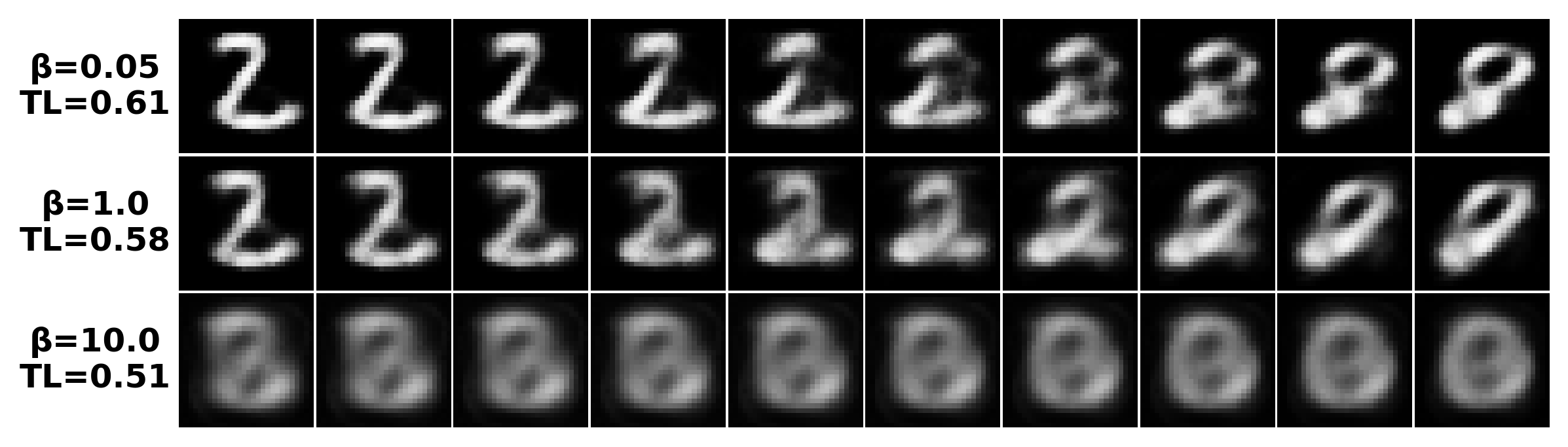
Linear interpolation in generative models
If the latent codes have high TL with respect to the inputs, a decoder can interpolate linearly in latent space.
Its interpolation error is bounded by the linear-regression reconstruction error. Lower \(\beta\) gives higher TL and cleaner 2→8 transitions. (Proposition 4)
More in the paper: TL across layers of pre-trained and fine-tuned BERT, TL under random labels and grokking,
CNN/ResNet whitening, and Adam.
Citation
@article{cha2026weight,
  title={The Weight Gram Matrix Captures Sequential Feature Linearization in Deep Networks},
  author={Cha, Taehun and Beaglehole, Daniel and Radhakrishnan, Adityanarayanan and Lee, Donghun},
  journal={arXiv preprint arXiv:2605.06258},
  year={2026}
}